Path Finding Modules
The Path Finding Modules (PFMs) are algorithms for converting images into geometric shapes, they can be configured in the Path Finding Controls panel. They have been designed to be as flexible as possible and to run with almost any combination of settings. This means that they can create many more styles than those you see here. Some of these extra styles are included as presets!
Every Path Finding Module can also be run with CMYK Separation
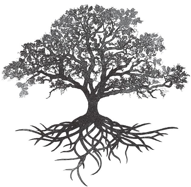
Sketch PFMs
Sketch PFMs are best used for plots using multiple layers of different pens as the Sketch PFMs rely on the different pens to represent the different tones in the image. However, it is possible to use a single pen with Sketch PFMs though it is recommended to use a pen which is additive where overlapping strokes will result in progressively darker lines.
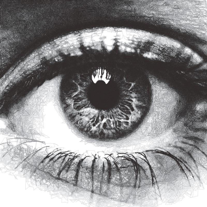
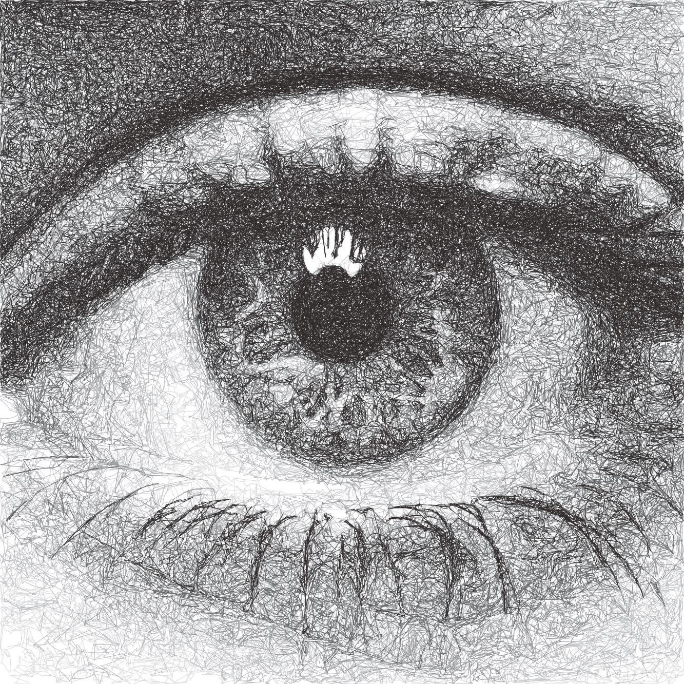
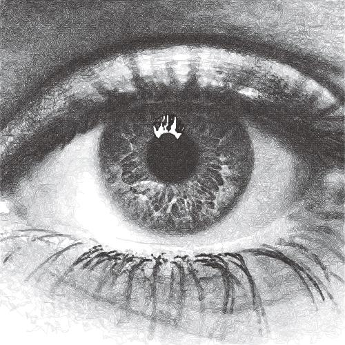
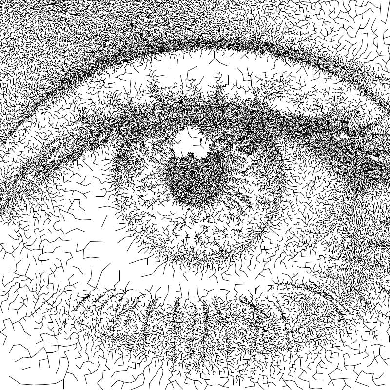
Sketch Lines
Transforms an image into lines using brightness data.
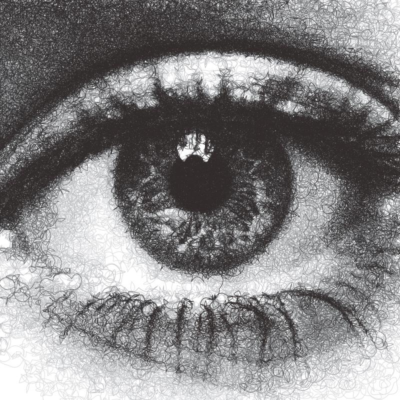
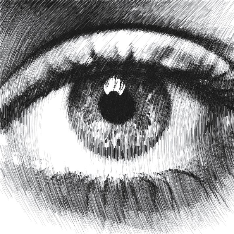
Sketch Curves
Transforms an image into catmull-rom splines using brightness data.

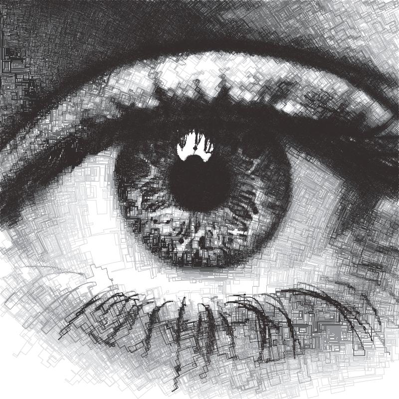
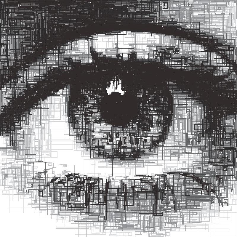
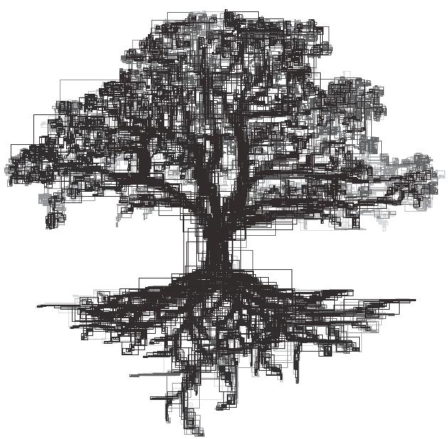
Sketch Squares
Transforms an image into lines in a rectangular pattern using brightness data.
Sketch Quad Beziers
Transforms an image into Quadratic Bézier curves using brightness data, by first finding the darkest line and then finding the darkest position for one control point. It uses more accurate “Bresenham” calculations which results in longer processing times but increased precision.
Sketch Cubic Beziers
Transforms an image into Cubic Bézier curves using brightness data, by first finding the darkest line and then finding the darkest position for the two control points. It uses more accurate “Bresenham” calculations which results in longer processing times but increased precision.
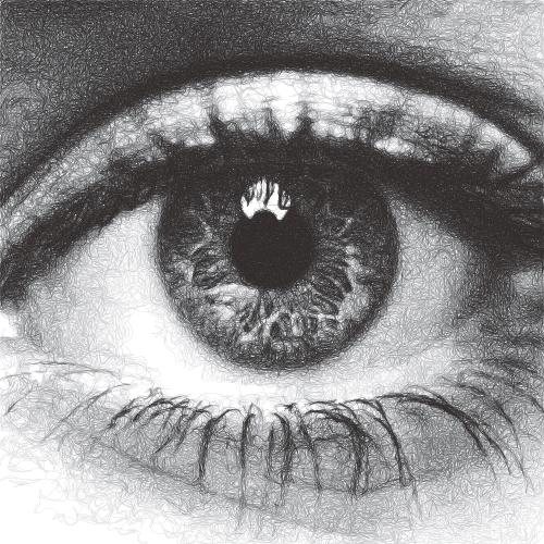
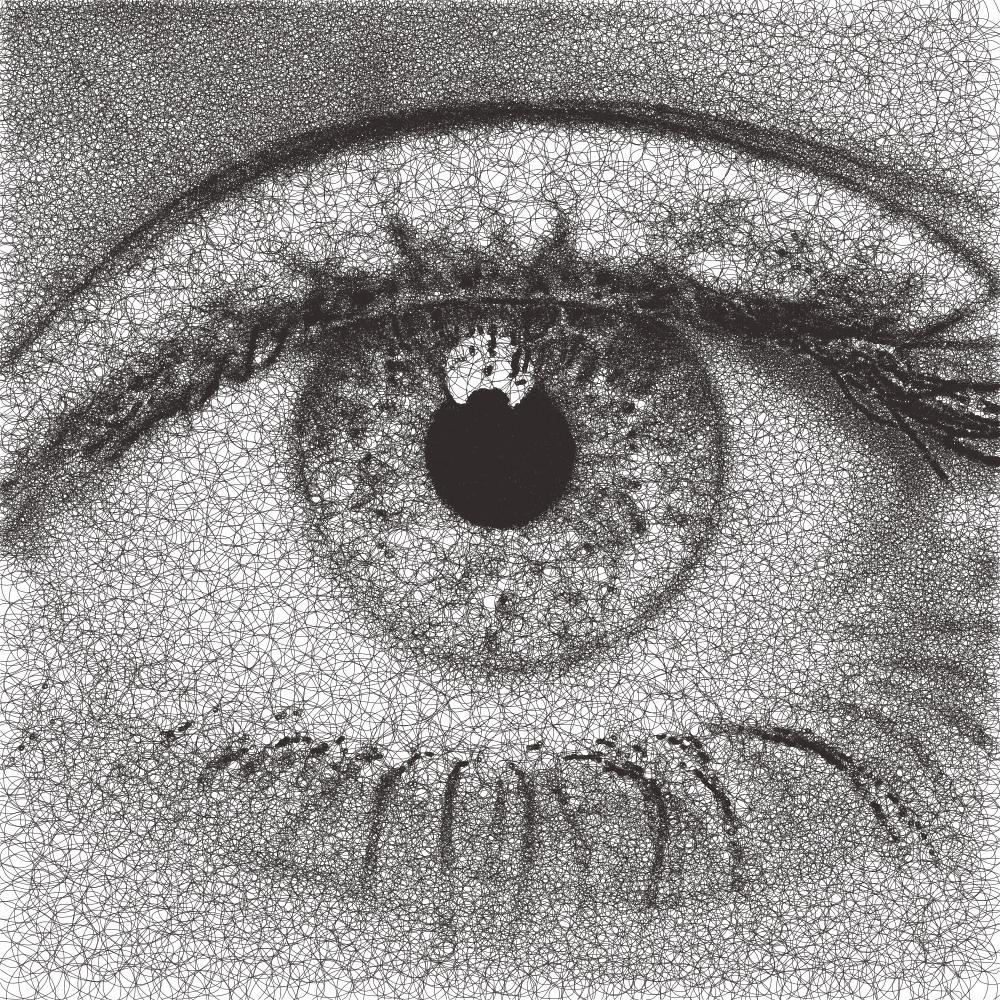
Sketch Catmull-Roms
Transforms an image into catmull-rom splines using brightness data, by finding the next darkest curve from each point. It uses more accurate “Bresenham” calculations which results in longer processing times but increased precision.
Sketch Shapes
Transforms an image into shapes using brightness data. It has the following modes: Rectangle and Ellipse. It uses a more accurate “Bresenham” calculation when considering each shape.
Sketch Sobel Edges
Transforms an image into lines using brightness data & edge detection data. By using a Sobel Operator to find sharp edges and then using this data in conjunction with the brightness to find the next line.
Sketch Waves
Transforms an image into lines which follow the direction defined by an X and Y curve function.
How they work
Find the darkest area of the image
Find the darkest pixel in that area
Finds the next darkest line from that pixel
Brighten the part of the image that the line covers
Repeat steps 2 to 4 until the specified squiggle length is reached then return to step 1
The process will stop when either the specified line density or max line limit has been reached.
Settings: All
Default
Plotting Resolution: the factor the original image is scaled by before plotting. Useful in reducing the number/density of lines, also decreased computation time.
Random Seed: used to generate all the random numbers used by the PFM. This means plots will always produce the same results.
Style
Should lift pen: if the pen should be raised when moving to the next darkest area, disabling this can create some unique styles
Directionality: forces the lines to follow the natural contours of the image
Distortion: adds some noise to the generated lines, creating more stylised images.
Angularity: higher angularity results in lines which don’t change direction as frequently, resulting in more sweeping curves in curve pfms
Edge Power: used to exaggerate key edges in the image
Sobel Power: used to exaggerate a cartoonish quality for the plot
Luminance Power: typically PFMs will follow dark areas in the image when creating lines, this slider can be used to decrease the influence of brightness which in turn will favour other style options like Directionarity or Edge Power etc.
Segments
Line Density: affects the total number of lines and therefore the computation time
Line Min Length: the minimum length of each line
Line Max Length: the maximum length of each line
Line Max Limit: limits the total number of lines, will only have an effect if this limit is reached before the chosen line density
Angle Tests: how many drawing angles to test before choosing the darkest line, increase this value to improve the accuracy of the plot, this will increase computation time.
Unlimited Tests: will run as many angle tests as required to find the “best” line possible, resulting in more accurate drawings with longer processing times.
Squiggles
Squiggle Min Length: prevents incredibly short squiggles from being created, shortening plotting times
Squiggle Max Length: defines the total number of connected lines which should be drawn before looking for the next darkest area of the image
Squiggle Max Deviation: allows you to control how far a squiggle is allowed to deviate in brightness before it is ended prematurely, this has the result of making shorter squiggles which are more accurate and less likely to cross over brighter areas of the image. Increasing the allowed deviation will result in a less accurate drawing with fewer pen lifts.
Generic
Adjust Brightness: the amount to change the pixel’s brightness by in the source image when a line is drawn, affects how often the PFM will draw over the same area.
Settings: Lines & Curves Only
Start Angle (Min & Max): the start angle affects the trajectory of lines, this has less effect when shading is disabled.
Shading: when shading is enabled the PFM will draw lines which are limited by the start angle min/max creating a diagonal shading effect
Shading Threshold: the point in the processing when shading will kick in, note this ignores max line limit
Drawing Delta Angle: the degrees of rotation that the PFM will use when finding the next line while drawing
Shading Delta Angle: the degrees of rotation that the PFM will use when finding the next line while shading
Settings: Curves & Catmull-Roms Only
Curve Tension: affects the tension of the catmull-rom splines,
0.0 = No Tension, unpredictable curves
0.5 = Medium Tension, smooth curves
1.0 = Maximum tension, straight lines.
Settings: Quad & Cubic Beziers Only
Curve Tests: the number of positions to test for each control point to find the darkest curve, increasing this will result in a more accurate plot.
Curve Variation: the maximum magnitude of the curve, increasing this will decrease the test accuracy and increase the control points offsets.
Curve Offset: allow you to control the ‘wiggle’ of the curve.
Settings: Shapes Only
Shape Type: Allows you to choose the type of shapes to draw the image with, current options = Rectangles, Ellipses
Settings: Sobel Edges Only
Sobel Intensity: the priority of edge detection vs brightness
Sobel Adjust: similar to adjust brightness, the amount to decrease a pixel’s sobel value by when a line is drawn over it, affects how strongly the PFM is affected by the sobel values.
Settings: Waves Only
Start Angle: Affects the rotation of the waves, useful to alter the results without dramatically changing the form of the waves.
Wave Offset X/Y: Shifts the X/Y wave across the image.
Wave Divisor X/Y: Affects the intensity of the X/Y wave, increasing the divisor will result in flatter waves, decreasing it will result in more exaggerated waves
Wave Type X/Y: Changes the mathematical wave used to create the wave, options: SIN, COS, TAN
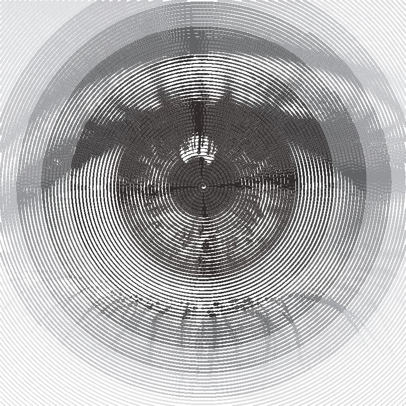
Spiral PFM
Transforms an image into a oscillating spiral using brightness data.
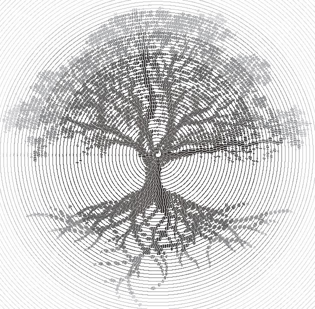
How it works
Moves to the first point on the spiral.
Samples the brightness at the current point and draws a line which is perpendicular to the spiral where the lines length is proportional to the sampled brightness.
Move to the next point on the spiral and Repeat step 2.
The process stops when the specified spiral size has been reached
Settings
Plotting Resolution: the factor the original image is scaled by before plotting. Useful in reducing the number/density of lines, also decreased computation time.
Random Seed: used to generate all the random numbers used by the PFM. This means plots will always produce the same results.
Spiral Size: the size of the generated spiral, a spiral at 100% will just touch the edge of the image.
Centre X: the x position of the centre point of the spiral as a percentage.
Centre Y: the y position of the centre point of the spiral as a percentage.
Ring Spacing: the distance between each generated ring
Amplitude: the scale of the oscillations
Density: may change a large density will result in less lines / brightness samples
Ignore White: When enabled the spiral won’t be drawn over areas which are white in the reference image.
Adaptive PFMS
‘Adaptive’ are named after the way they adapt to match the tone of the input image.
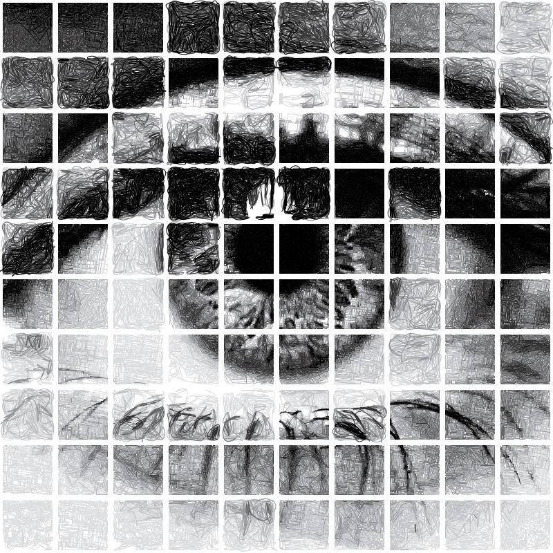
This means the reproductions of tones is way more accurate then other PFMs, this means they have an additional processing stage “Tone Mapping”. This process only needs to be performed once per configuration of settings, if you change a setting which could alter the tone map it will run again.
You can view the output of the tone mapping stage by selecting “Display:” and then “Tone Map”, this shows you three outputs the Reference Tone Map, the drawing created by the PFM with the current settings and the blurred version of this output.
For the best results with Adaptive PFMs use high resolution, high contrast images
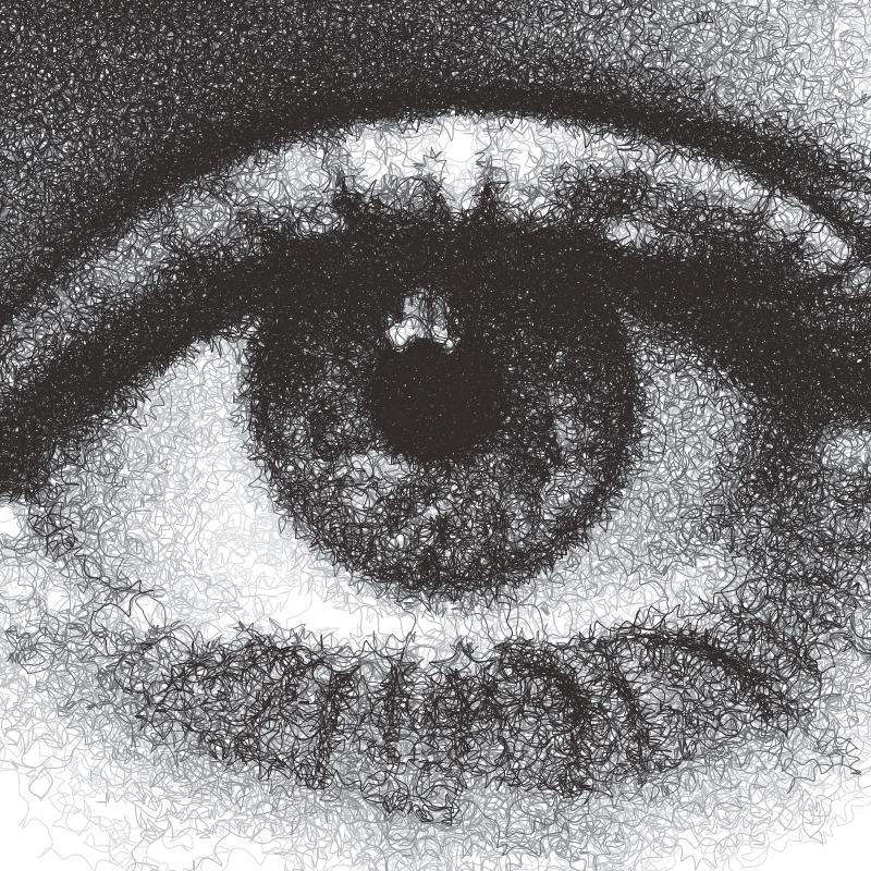
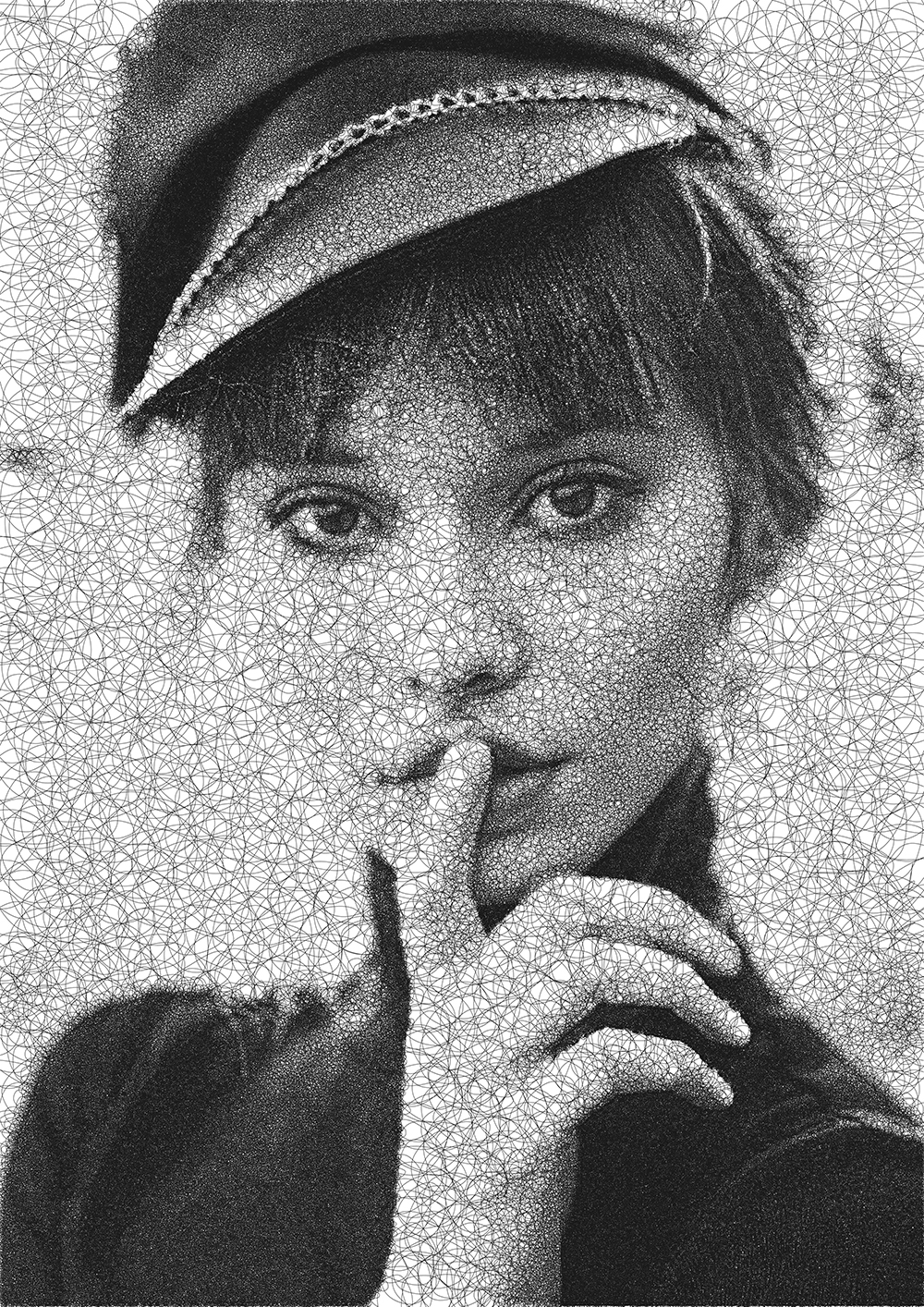
Adaptive Circular Scribbles
Transforms an image into a single continuous circular scribble.
This is an implementation of Chiu Et Al 2015, “Tone‐ and Feature‐Aware Circular Scribble Art”. If you wish to achieve results similar to Chiu Et Al’s implementation use a size of paper, pen width which gives you a plotting size of 4000px on the largest edge then use the “Chiu Et Al – 4000px” preset
Adaptive Shapes
Transforms an image into a series of packed shapes
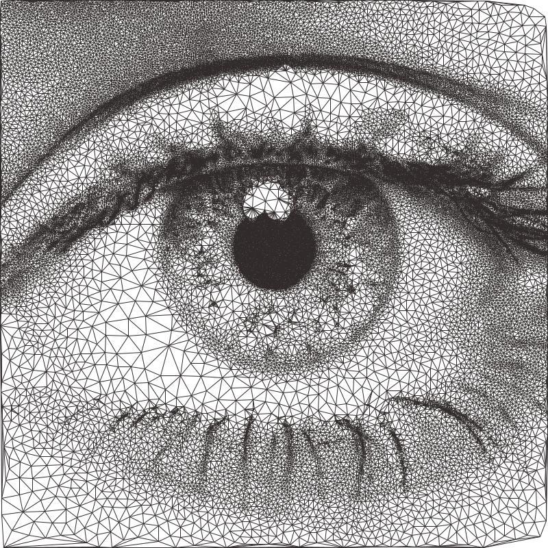
Adaptive Triangulation
Transforms an image into a series of connected triangles joining all the points generated using Delaunay Triangulation
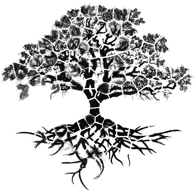
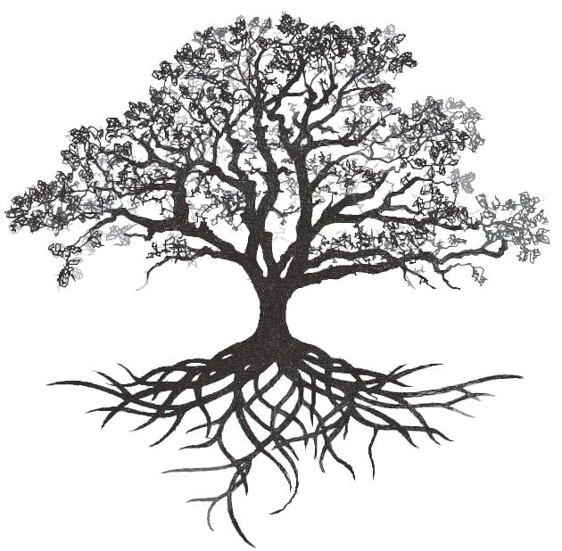
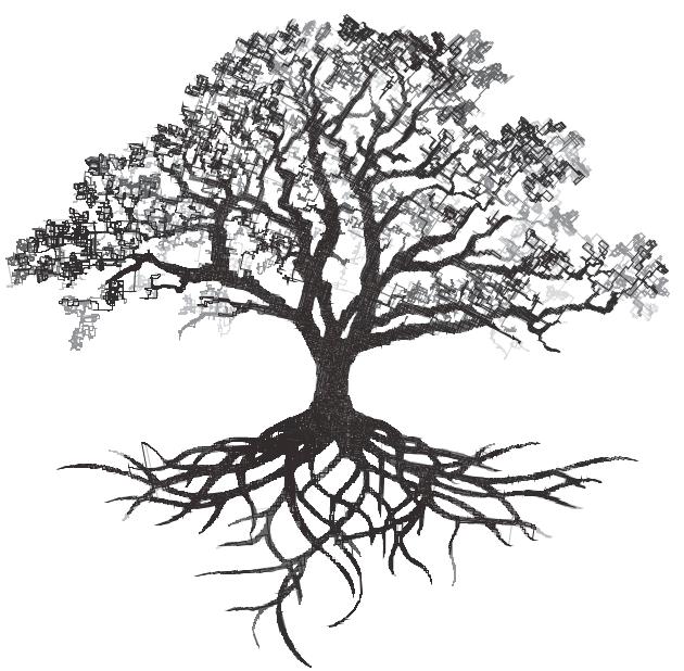
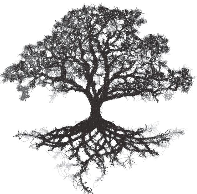
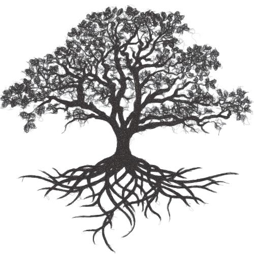
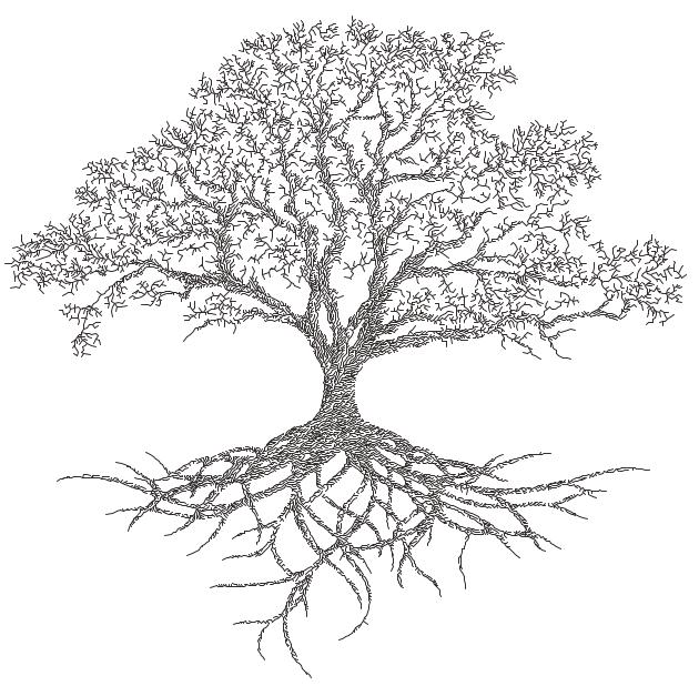
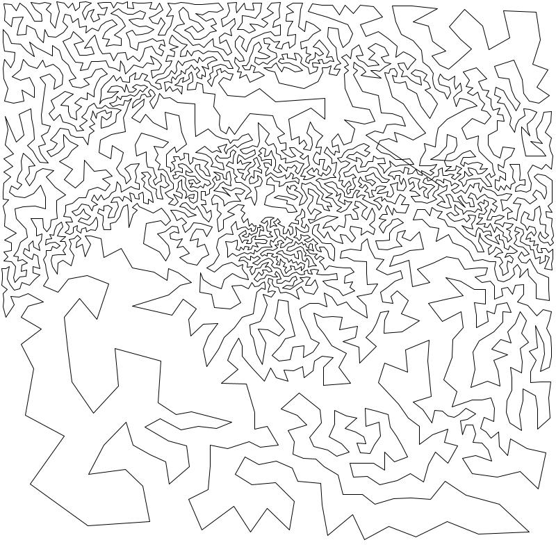
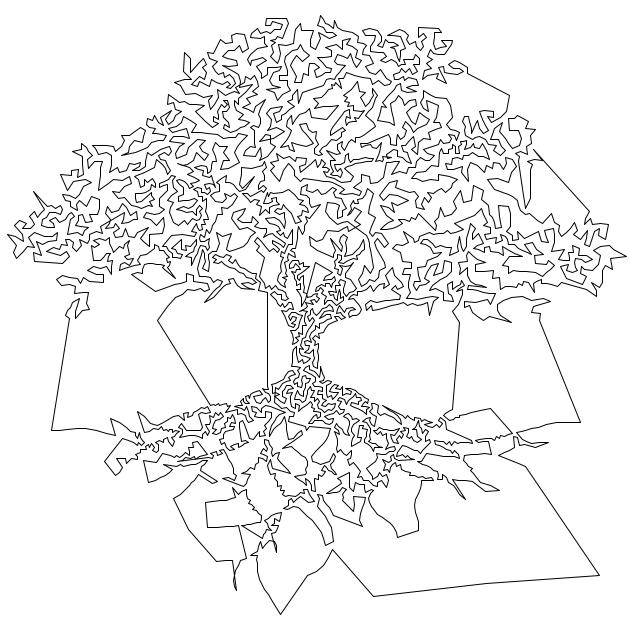
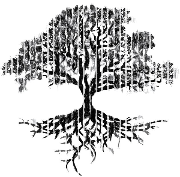
Adaptive Tree
Transforms an image into a Minimum Spanning Tree, which connects all the points generated into a minimum length tree.
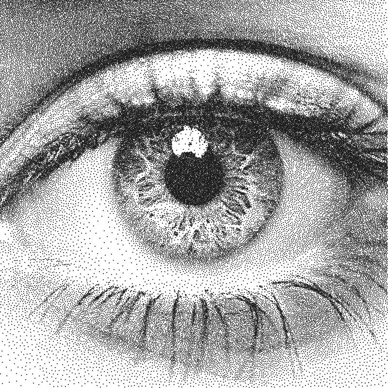
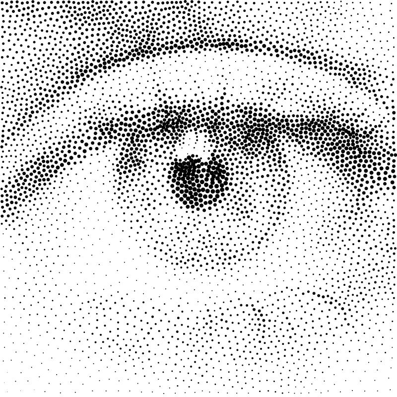
Adaptive Stippling
Transforms an image into a series of dots placed at each point generated.
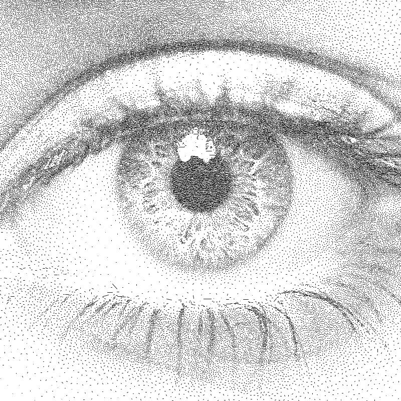
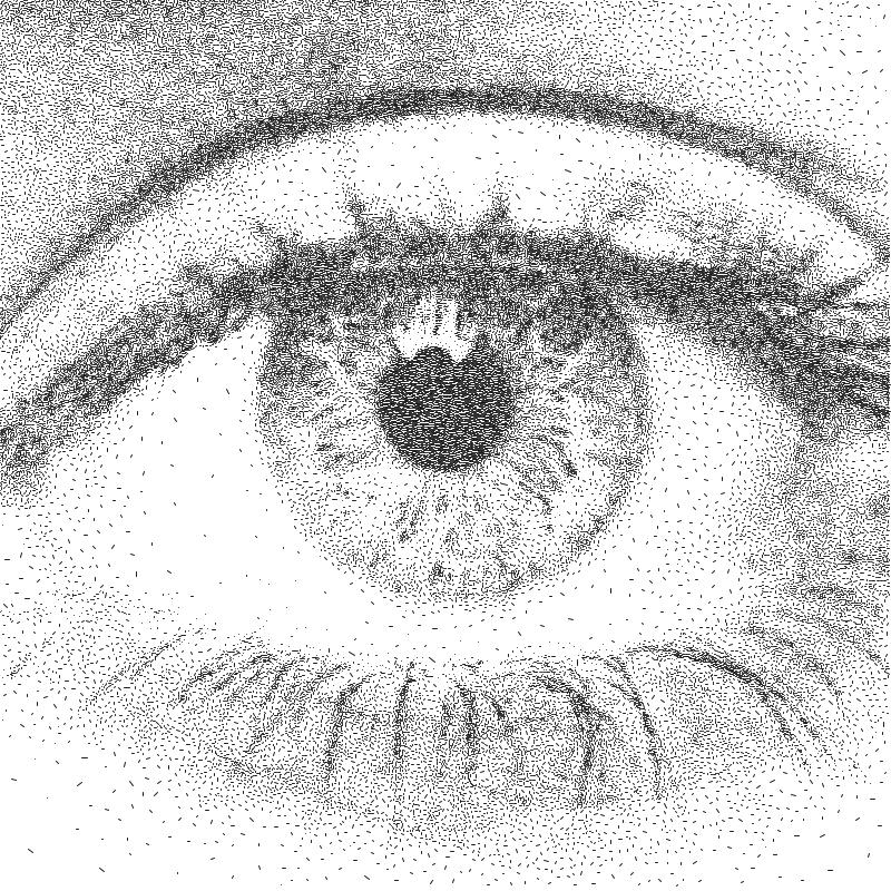
Adaptive Dashes
Transforms an image into a series of dashes placed at each point generated.
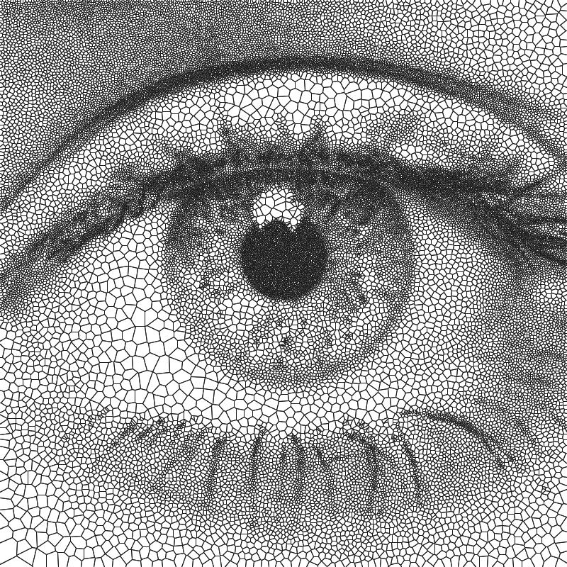
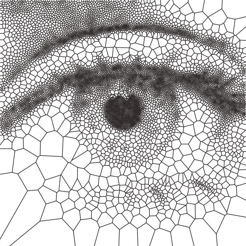
Adaptive Diagram
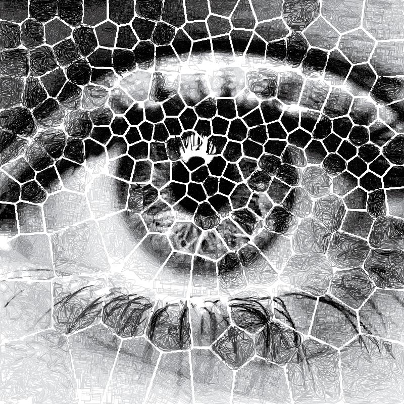
Transforms an image into a Voronoi Diagram which is generated from all of the evenly distributed points.
Adaptive TSP
Transforms an image into a one continuous line, or alternatively multiple individual continuous line segments.

How they work
Generate a Tone Map using steps 2 to 3, analyse the result then create a new input image which will result in drawing with a more accurate representation of the original tones.
Create evenly distributed points across the image based on brightness.
Generate the specific style based on these points.
Voronoi PFMs
All Voronoi PFMs utilise a Weighted Voronoi Diagram to determine the distribution of brightness in the original image and then use this diagram to generate new styles.
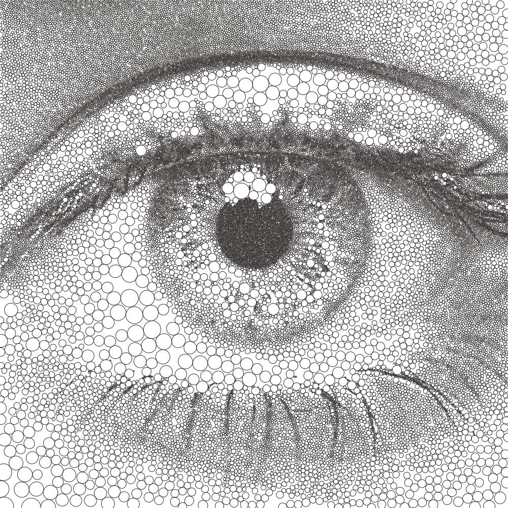
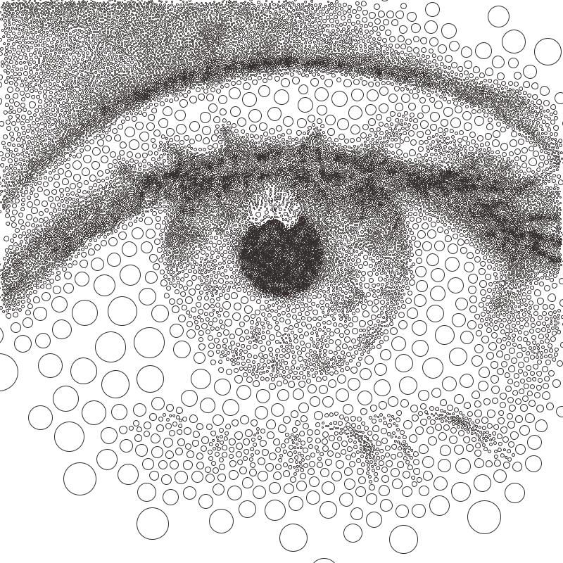
Voronoi Circles
Transforms an image into a series of inscribed circles for each cell of the voronoi diagram.
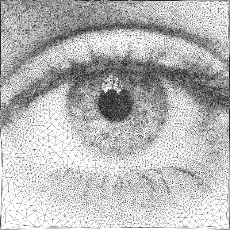
Voronoi Triangulation
Transforms an image into a series of connected triangles joining all the centroids in the voronoi diagram using Delaunay Triangulation

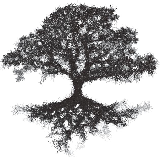
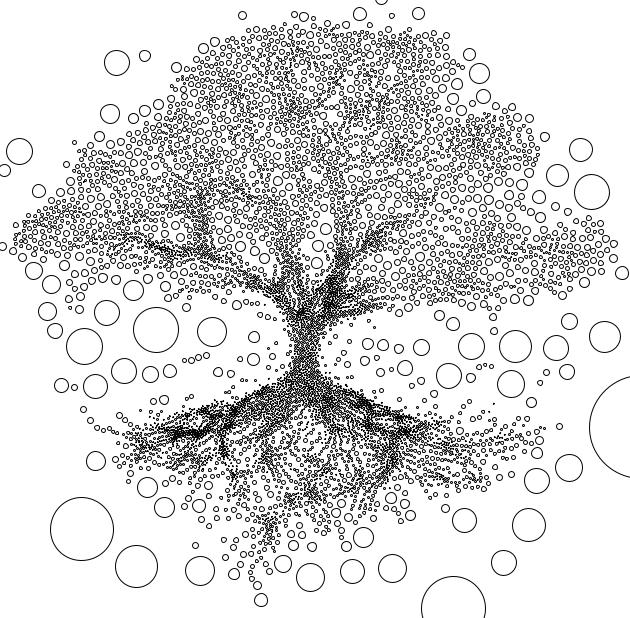
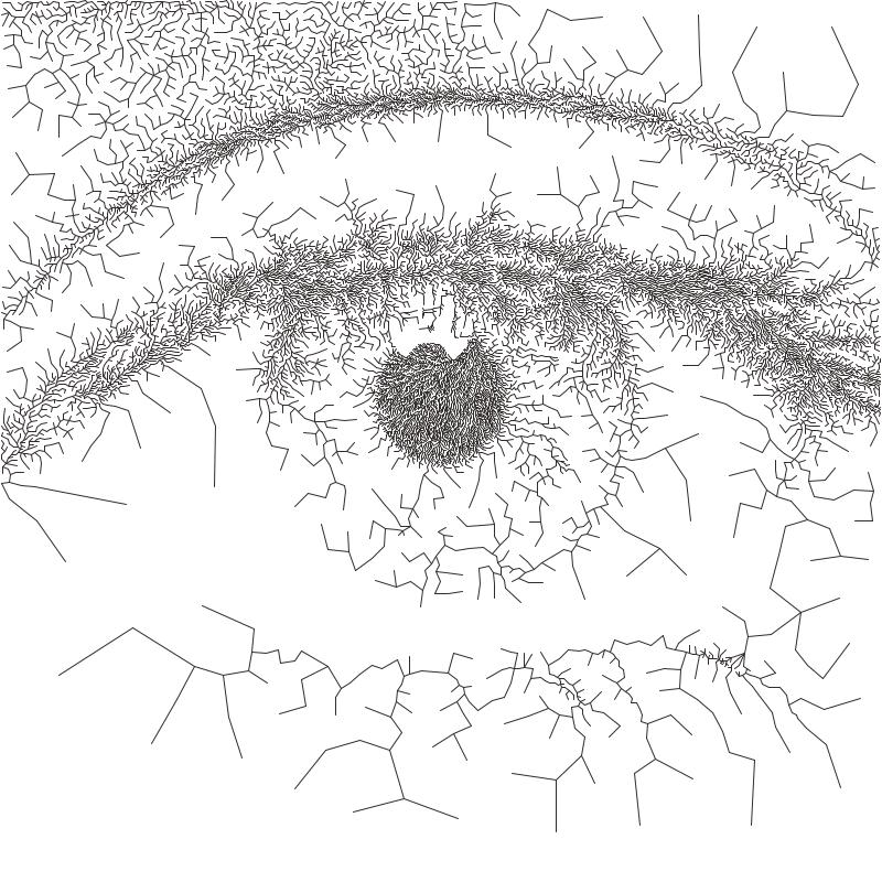
Voronoi Tree
Transforms an image into a Minimum Spanning Tree, which connects all the centroids in the voronoi diagram into a minimum length tree.
Voronoi Stippling
Transforms an image into a series of filled circles for each centroid in the voronoi diagram, the size of the “stipple” is relative to the sampled brightness of the cell the centroid belongs to.

Voronoi Dashes
Transforms an image into a series of dashes at each centroid in the voronoi diagram.
Voronoi Diagram
Transforms an image into a Voronoi Diagram

Voronoi TSP
Transforms an image into a series of connected lines for each centroid in the voronoi diagram with the shortest distance. By solving the Travelling Salesman Problem.
How they work
Randomly scatter points over the image proportional to the images brightness
Calculates a voronoi diagram based on these points.
Calculates the weighted centroids of each cell in the diagram using brightness data.
Use the generated centroids to re-calculate the voronoi diagram.
Return to step 3
The process finishes when the specified number of voronoi iterations have been performed.
Settings: All
Plotting Resolution: the factor the original image is scaled by before plotting. Useful in reducing the number/density of lines, also decreased computation time.
Random Seed: used to generate all the random numbers used by the PFM. This means plots will always produce the same results.
Point Count: the number of cells of the underlying voronoi diagram / how many points to scatter in step 1.
Luminance Power: used when randomly scattering points over the image, it affects how bias the scattering is towards darker areas of the image, typically using the same value for Density Power yields the best results.
Density Power: used when calculating the centroids of the voronoi diagram, it affects the calculation’s bias towards darker areas of the image, typically using the same value for Luminance Power yields the best results.
Voronoi Iterations: how many times to re-calculate the voronoi diagram, more iterations will result in a more accurate representation of the original image.
Settings: Circles Only
Circle Size: the fill percentage of each circle where 100% is the largest circle which still fits within it’s voronoi cell.
Settings: Triangulation Only
Triangulate Corners: when enabled the PFM will add triangles which connect the corners of the image to the other points
Settings: Stippling Only
Stipples Size: the fill percentage of each stipple where 100% is the maximum size of the stipple relative to the image’s brightness
Mosaic PFMs
Mosaic PFMs offer different ways to split an image into different sections which can then be passed through different PFMs to create a Mosaic effect.
Mosaic Rectangles
Divides an image into a series of rectangles which can are then distributed randomly amongst the enabled Drawing Styles
Mosaic Voronoi
Divides an image into a Voronoi Diagram, each cell is distributed randomly amongst the enabled Drawing Styles